Notes on rl in finance book
These are my notes as I read through the Foundations of reinforcement learning book by Ashwin Rao and Tikhon Jelvis.
Chapter 1
The first chapter basically about coding and designing programs. The book has code samples (written in python) within it with explanations of the concepts relevant to RL. All the code used in the book is available on the GitHub page.
Chapter 2
Defines basic concepts of sequential decision making.
Markov states - they have the property that the probabilities of state St + 1 only depends on the current state St. This is commonly states as “the future is independent of the past given the present”
Formally a Markov process consists of
- a countable set of states S known as the state space. terminal states are a subset of the state space
- time-indexed sequence of random states St with each transition satisfying the markov property
Usually it is assumed that the transition probability matrix, which defines the probability of St moving to St + 1 , is stationary i.e it does not change with time t . Otherwise it would make the job of the modeler significantly more difficult.
One interesting question introduced here is how do we start the markov process? Is the starting position arbitrary or does it follow some specific probability distribution?
There is a very good example of modelling inventory management as an MDP.
Assume that you are the owner of a bicycle shop and need to order bicycle to meet the demand. The demand is random, but it follows a Poisson distribution. There are constraints on the storage space so you can store at most C . Any order you place arrives after 36 hours i.e lead time of 36 hours.
α is the on-hand inventory and β is the on-order inventory.
The state St , is defined as the inventory position at 6 pm each day. You close the store at 6 and just before closing review the inventory and order additional units if required. The policy that you follow is to order C - (α + β) if your inventory position is less than the capacity constraint. If the inventory position is greater than the store capacity, no order will be placed.
This is modelled as a markov process with the sales of the bicyles being the random variables. A transition function is defined that maps the current inventory position to a a future inventory position. The sales are random and sampled from a poisson distribution. To illustrate the transition probabilities they have a very nice illustration.
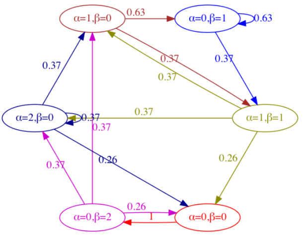
Assuming that the storage capacity is 2 and we begin the markov process with an empty store, we would immediately order 2 bicycles. Then there is 37% probability that the next state is with 2 bicycles in the store. Then there is a 37% probability that no sales are recorded on that day resulting in a self-loop. 26% probability that you sell of the 2 bicycles and end up in the start state with no bicycles in the store and none on order.
Markov reward processes include a notion of a numerical reward to the markov process. The rewards are given for each state transition. They are ransom and need to be specified with the probability distribution of these rewards. A discount factor is applied to future rewards. Introducing the concept of markov reward process to the inventory example we get a holding cost for all the bicycles that remain in the store overnight and a stockout cost that is incurred whenver demand is missed due to insufficient inventory. Usually significantly more weight is given to the stockout cost than the holding cost.
Value functions
Value functions form the core the core of most reinforcement learning applications. Value functions are functions of states or state-action pairs that estimate how good it is for the agent to be in a given state.